
Why Use NumPy?
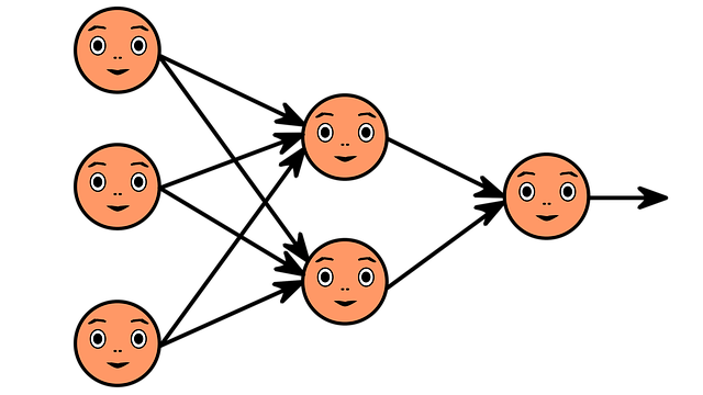
In the previous articles, we built an artificial neuron and a simple layer using pure Python code. The logic was not complicated: weighted sum, add bias, and optionally apply an activation function.
But as networks grow larger — with multiple layers and hundreds or thousands of neurons — pure Python solutions become:
- slow,
- hard to manage,
- and prone to errors.
This is why we use the NumPy library, which is:
- very fast (written in C language),
- reliable (thoroughly tested),
- and makes vector and matrix operations easy.
Vectors, Arrays, Matrices and Tensors
Before we look at how NumPy is used through specific examples, it is important to clarify a few concepts.
Let's start with the simplest Python data store, the list. A Python list contains comma-separated numbers enclosed in square brackets. In the previous sections, we used lists to store data in our pure Python solutions.
Example of a list:
list = [1, 5, 6, 2]List of lists:
list_of_lists = [[1, 5, 6, 2],
[3, 2, 1, 3]]List of lists of lists:
list_of_lists_of_lists = [[[1, 5, 6, 2],
                           [3, 2, 1, 3]],
                          [[5, 2, 1, 2],
                           [6, 4, 8, 4]],
                          [[2, 8, 5, 3],
[1, 1, 9, 4]]]All of the above examples can also be called arrays. However, not all lists can be arrays.
For example:
 [[1, 2, 3],
   [4, 5],
[6, 7, 8, 9]]This list cannot be an array because it is not "homologous". A "list of lists" is homologous if each row contains exactly the same amount of data and this is true for all dimensions. The example above is not homologous because the first list has 3 elements, the second has 2, and the third has 4.
The definition of a matrix is simple: it is a two-dimensional array. It has rows and columns. So a matrix can be an array. Can every array be a matrix? No. An array can be much more than rows and columns. It can be 3, 5, or even 20 dimensions.
Finally, what is a tensor? The exact definition of tensors and arrays has been debated for hundreds of pages by experts. Much of this debate is caused by the participants approaching the topic from completely different areas. If we want to approach the concept of tensor from the perspective of deep learning and neural networks, then perhaps the most accurate description is: "A tensor object is an object that can be represented as an array."
In summary: A linear or 1-dimensional array is the simplest array, and in Python, a list corresponds to this. Arrays can also contain multidimensional data, the most well-known example of which is a matrix, which is a 2-dimensional array.
One more concept that is important to clarify is the vector. Simply put, a vector used in mathematics is the same as a Python list, or a 1-dimensional array.
Two Key Operations: Dot Product and Vector Addition
When performing the dot product operation, we multiply two vectors. We do this by taking the elements of the vectors one by one and multiplying the elements with the same index, then adding these products. Mathematically, this looks like this:
\vec{a}\cdot\vec{b} = \sum_{i=1}^n a_ib_i = a_1\cdot b_1+a_2\cdot b_2+...+a_n\cdot b_nIt is important that both vectors have the same size. If we wanted to describe the same thing in Python code, it would look like this:
# First vector
a = [1, 2, 3]

# Second vector
b = [2, 3, 4]

# Dot product calculation
dot_product = a[0]*b[0] + a[1]*b[1] + a[2]*b[2]

print(dot_product)

>>> 20
You can see that we have performed the same operation as when calculating the output value of a neuron, only here we have not added the bias. Since the Python language does not contain any instructions or functions for calculating the dot product by default, we use the NumPy library.
When adding vectors, we add the elements of each vector with the same index. Mathematically, this looks like this:
\vec{a}+\vec{b} = [a_1+b_1, a_2+b_2,...,a_n+b_n]Here again, it is important that the vectors have the same size. The result will be a vector of the same size. NumPy handles this operation easily.
Using NumPy
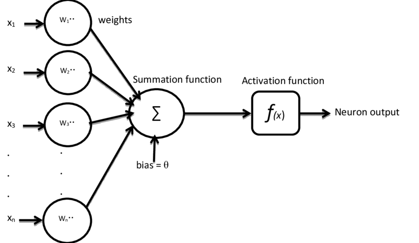
A neuron
Let’s now implement a neuron using NumPy.
import numpy as np

# Inputs and weights
inputs = np.array([0.5, 0.8, 0.3, 0.1])

weights = np.array([0.2, 0.7, -0.5, 0.9])

bias = 0.5

# Neuron output (dot product + bias)
output = np.dot(inputs, weights) + bias

print("Neuron output:", output)
Here, np.dot(inputs, weights) computes the dot product, and then we simply add the bias.
A layer
Now let’s build a layer of 3 neurons, each receiving 4 inputs.
import numpy as np

# Example inputs (4 elements)
inputs = np.array([1.0, 2.0, 3.0, 2.5])

# Weights for 3 neurons (matrix: 3 rows, 4 columns)
weights = np.array([
                [0.2, 0.8, -0.5, 1.0],       # Neuron 1
                [0.5, -0.91, 0.26, -0.5],    # Neuron 2
                [-0.26, -0.27, 0.17, 0.87]   # Neuron 3
])

# Bias values (3 elements)
biases = np.array([2.0, 3.0, 0.5])

# Layer output (matrix multiplication + vector addition)
output = np.dot(weights, inputs) + biases

print("Layer output:", output)

>>> Layer output: [4.8   1.21  2.385]
Here, np.dot(weights, inputs) computes the matrix-vector product, which is exactly the weighted sum for each neuron. Adding the bias vector completes the computation.
Next Article
In the next article, we will explore activation functions, and see how they provide the "nonlinear power" that makes neural networks much more capable. Without them, our network would only be able to model simple linear relationships.