
In the previous parts, we built a layer that computes the raw output of neurons – the weighted sum plus bias. However, that output is linear: if you double the input, the output doubles. A linear network can only learn straight-line relationships.
But the real world is nonlinear. Image recognition, speech understanding, and natural language processing all involve complex patterns that linear models cannot capture. This is where activation functions come in. These nonlinear transformations give neural networks the ability to sense, adapt, and truly learn.
The Role of Activation Functions
Without activation:
output = sum (inputs * weights) + bias
With activation:
output = f(sum (inputs * weights) + bias)
The function f() is the activation function, and it’s what gives the network its learning power.
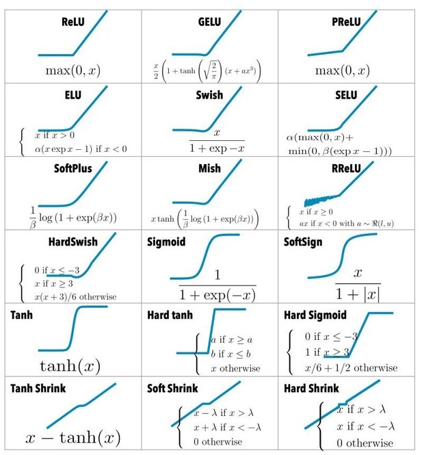
Common Activation Functions
Step Function
The simplest of all activation functions is the Step. It works like a switch: if the neuron’s input is above a threshold, the output is 1; otherwise, it’s 0.
f(x) = \begin{cases} 1 & \text{ } x \geq 0 \\ 0 & \text{ } x < 0 \end{cases}Graphically depicted:
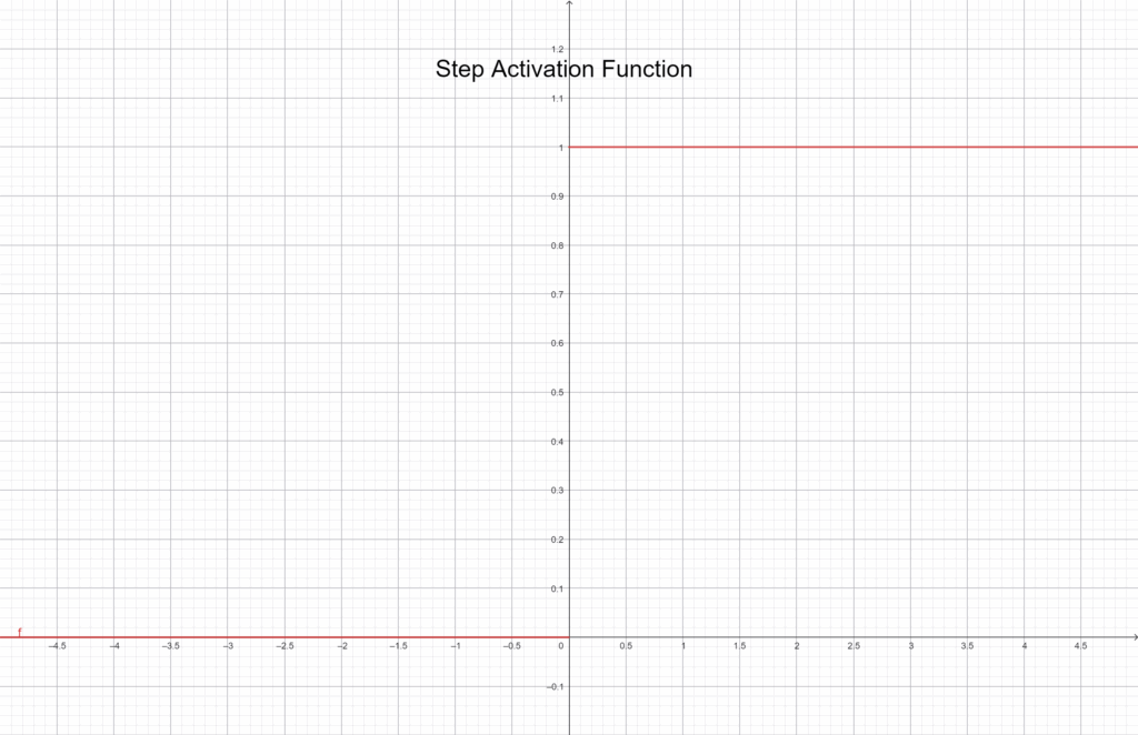
It’s a good way to illustrate how neurons turn on or off, but it’s not suitable for training, since it’s not continuous and doesn’t support gradient-based learning. Step is mostly used for demonstration purposes, as we did earlier.
Sigmoid Function
The Sigmoid is smoother. It squashes every input into the range 0–1 following a soft S-shaped curve:
f(x) = \frac {1} {(1 + e^{-x})}Graphically depicted:
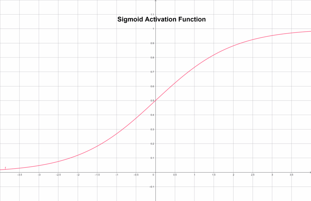
This makes it ideal when we want an output that represents probability, such as in binary classification tasks. However, the Sigmoid’s gradient becomes extremely small for very large or small input values, slowing down learning — a problem known as the vanishing gradient.
Tanh Function
The tanh function, short for hyperbolic tangent, is similar to Sigmoid but scales outputs between -1 and 1:
f(x) = tanh(x)
Graphically depicted:
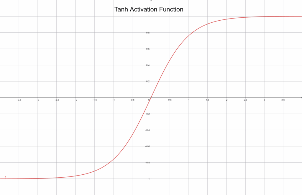
Because its output is centered around zero, it often trains faster and more stably. Still, it suffers from the same vanishing gradient issue in extreme regions. Despite that, it remains popular in smaller or older networks for its intuitive and balanced behavior.
ReLU (Rectified Linear Unit)
The ReLU is perhaps the most widely used activation function in modern networks. It’s defined as:
f(x) = max(0, x)
Graphically depicted:
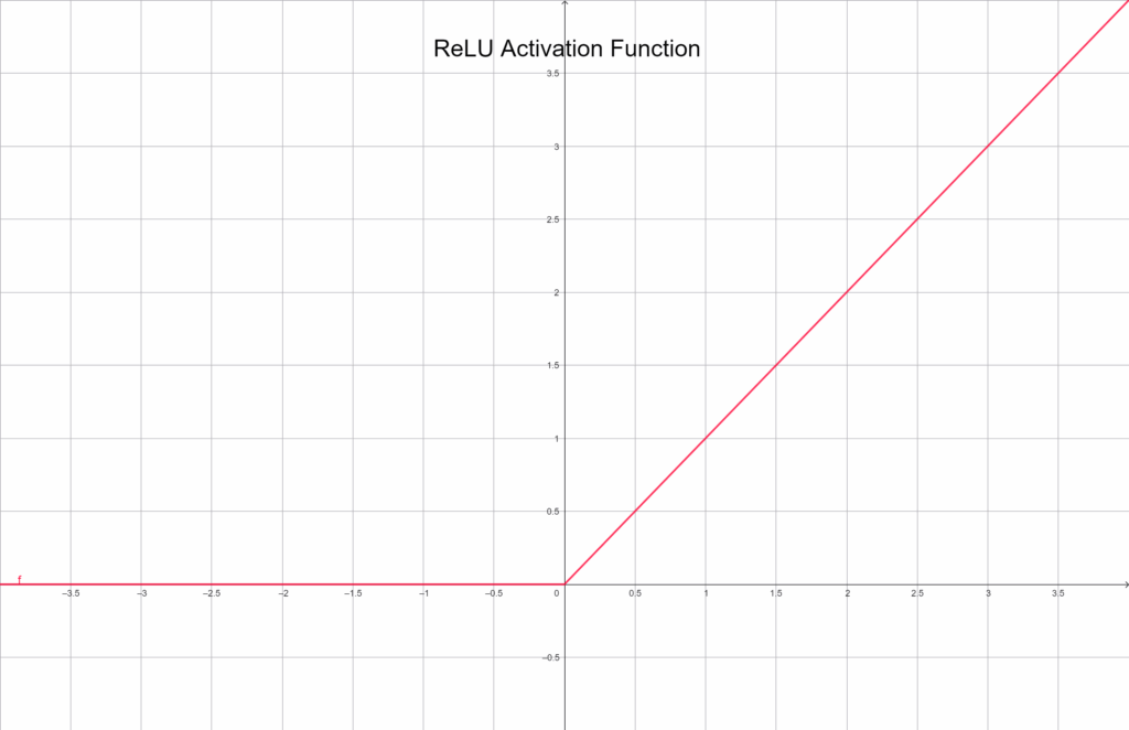
Negative inputs become 0, positive inputs pass through unchanged. Its simplicity is its strength — it’s fast, efficient, and avoids the Sigmoid’s gradient issues. However, some neurons can “die” if they get stuck with negative inputs forever, never activating again. Even so, ReLU remains the default choice for most deep learning models.
Leaky ReLU
The Leaky ReLU improves on ReLU by allowing a small, nonzero output for negative inputs:
f(x) = \begin{cases} x & \text{ } x \geq 0 \\ 0.01*x & \text{ }x < 0 \end{cases}Graphically depicted:
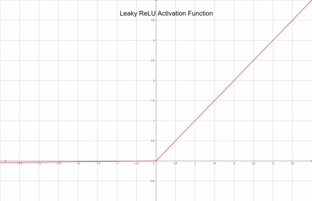
This tiny “leak” keeps neurons alive even when their inputs are mostly negative, leading to more stable training. It’s often used when too many neurons become inactive under standard ReLU.
Summary
Activation functions give neural networks their nonlinear power. Without them, a model could only describe linear relationships — essentially a flat plane or line. With them, neural networks can learn complex, nonlinear decision boundaries and perform genuinely intelligent behavior.
In the next article, we’ll see how to implement these activation functions in Python and NumPy, and observe how they transform a layer’s output in practice.